Differentiation vs. Integration

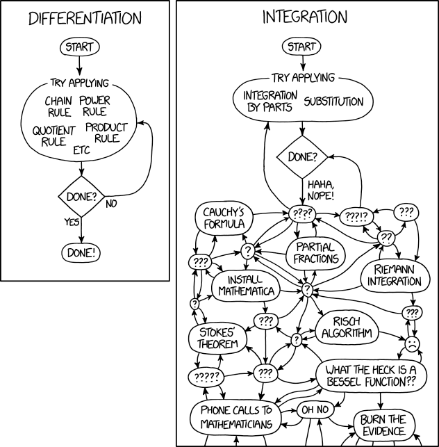
Recently, I posted a link to the above XKCD cartoon to social media and was asked if I could provide an explanation of why differentiation is relatively easy while integration is quite hard in comparison.

Differentiation:  Let's begin by laying out the ground rules.  We're interested in finding a formula for the derivative of a function given as a symbolic expression rather than computing a numerical approximation to the derivative of some function computed numerically (the latter problem is actually much harder in practice.)  We'll assume that our expression is written in terms of elementary operations: addition, subtraction, multiplication, division, powers (including roots), exponentials, logs,  trig functions (sin, cos, tan, and their inverses.)   We'll call a function \( f(x) \) elementary if it can be expressed in this way.

In your first semester of freshmen calculus, you learned a set of rules for computing derivatives that included rules for the derivatives of sums, products, and quotients of functions as well as trig functions, powers, exponentials, and logs.  Most importantly, you learned the chain rule for the derivative of the composition of two functions:

\( (f(g(x))'=f'(g(x))g'(x). \)

By applying these rules of differentiation recursively, you can systematically find the derivative of any elementary function.  Implementing symbolic differentiation in a functional programming language like Lisp makes for a nice homework exercise.

It's important to understand that these rules produce expressions that themselves are made up entirely of elementary functions.  Thus we say that the set of elementary functions is closed under differentiation.

Note that although the set of functions that can be produced by differentiation of elementary functions is contained in the set of elementary functions, it doesn't consist of all elementary functions- there are elementary functions that can't be reached by starting with an elementary function and differentiating it.

Integration:  Now suppose that we're given an expression written in terms of elementary functions and want to reverse the process to find its indefinite integral (also called the antiderivative.)  Definite integrals over an interval are also of interest, but they can be evaluated by using the antiderivative.

In second semester calculus, we teach students techniques of integration, which are basically heuristic procedures for reverse the process of differentiation step by step.  For example, the substitution method is simply a process for applying the chain rule:

\( \int f'(u(x)) u'(x) dx = f(u(x))+C \)

where \( C \) is an arbitrary constant  (whose derivative is 0.)

One difficulty in this approach to integration is that it isn't always clear which technique of integration should be applied.  Furthermore, it may be necessary to apply several of the techniques in order to fully evaluate the integral. 

A more significant problem is that it is possible to write down an elementary function that is not the derivative of any elementary function.   Therefore, the indefinite integral of such a function can't be written in terms of elementary functions. A famous example of this is

\( \int e^{-x^{2}} dx \).

A theorem due to Liouville gives conditions that determine whether or not an elementary function has an elementary antiderivative (Liouville had several theorems named after him- this is the one in differential algebra.)  Liouville's theorem is nontrivial to explain and in practice, it isn't possible to check the conditions by hand for most integrals.  Risch's algorithm is a systematic procedure that can distinguish between these cases and produce the integral when it is an elementary function.

Symbolic computation packages such as Maple and Mathematica used to evaluate integrals by the same kinds of heuristic techniques of integration that we teach to students in Calculus II.  More recently, these packages have incorporated more or less complete implementations of the Risch algorithm.  However, the algorithm is extremely difficult to fully implement and these packages can still fail to evaluate many integrals.  This is an area where human expertise is still quite valuable.

Users often want to see and understand the steps taken in evaluating an integral, but it's impractical to follow the steps of the Risch algorithm, so software packages offer evaluation by conventional techniques of integration with step by step descriptions.

Special Functions: Beyond elementary functions, there are also so-called "special functions" that are defined in terms of integrals or solutions of differential equations that cannot be expressed in terms of elementary functions.  For example, the complementary error function is defined as:

\( \mbox{erfc}(z)=\frac{2}{\sqrt{\pi}} \int_{z}^{\infty} e^{-x^{2}} dx \).

This function is useful in the statistical analysis of measurement errors.  We've already mentioned that \( e^{-x^{2}} \) is an example of a function that can't be integrated in terms of elementary functions.  However, there are many numerical methods for approximating this complementary error function and it is useful enough that it is commonly implemented in libraries of special functions.


Further Reading

Bronstein, Manuel. “Integration of Elementary Functions.” Journal of Symbolic Computation 9, no. 2 (February 1, 1990): 117–73. https://doi.org/10.1016/S0747-7171(08)80027-2.

Churchill, R. C. “Liouville’s Theorem on Integration in Terms of Elementary Functions.” In Lecture Notes for the Kolchin Seminar on Differential Algebra, 2002. https://ksda.ccny.cuny.edu/PostedPapers/liouv06.pdf.

Conrad, Brian. “Impossibility Theorems for Elementary Integration.” In Academy Colloquium Series. Clay Mathematics Institute, Cambridge, MA. Citeseer, 2005. http://citeseerx.ist.psu.edu/viewdoc/download?doi=10.1.1.482.3491&rep=rep1&type=pdf.

Cruz-Sampedro, Jaime, and Margarita Tetlalmatzi-Montiel. “Hardy’s Reduction for a Class of Liouville Integrals of Elementary Functions.” The American Mathematical Monthly 123, no. 5 (May 1, 2016): 448–70. https://doi.org/10.4169/amer.math.monthly.123.5.448.

Fitt, A. D., and G. T. Q. Hoare. “The Closed-Form Integration of Arbitrary Functions.” The Mathematical Gazette 77, no. 479 (July 1993): 227. https://doi.org/10.2307/3619719.

Geddes, K. O., S. R. Czapor, and G. Labahn. “The Risch Integration Algorithm.” In Algorithms for Computer Algebra, edited by K. O. Geddes, S. R. Czapor, and G. Labahn, 511–73. Boston, MA: Springer US, 1992. https://doi.org/10.1007/978-0-585-33247-5_12.

Kasper, Toni. “Integration in Finite Terms: The Liouville Theory.” SIGSAM Bull. 14, no. 4 (November 1980): 2–8. https://doi.org/10.1145/1089235.1089236.

Marchisotto, Elena Anne, and Gholam-Ali Zakeri. “An Invitation to Integration in Finite Terms.” The College Mathematics Journal 25, no. 4 (September 1994): 295. https://doi.org/10.2307/2687614.

Moses, Joel. “An Introduction to the Risch Integration Algorithm.” In Proceedings of the 1976 Annual Conference, 425–428. ACM ’76. New York, NY, USA: ACM, 1976. https://doi.org/10.1145/800191.805632.

Risch, Robert H. “The Problem of Integration in Finite Terms.” Transactions of the American Mathematical Society 139 (May 1969): 167. https://doi.org/10.2307/1995313.

Risch, Robert H. “The Solution of the Problem of Integration in Finite Terms.” Bulletin of the American Mathematical Society 76, no. 3 (May 1970): 605–8.

Ritt, Joseph Fels. Integration in Finite Terms: Liouville’s Theory of Elementary Methods. 1st edition. Columbia Univ. Press, 1948.

Rosenlicht, Maxwell. “Integration in Finite Terms.” American Mathematical Monthly, 1972, 963–972.

Rosenlicht, Maxwell. “Liouville’s Theorem on Functions with Elementary Integrals.” Pacific Journal of Mathematics 24, no. 1 (January 1, 1968): 153–61. https://doi.org/10.2140/pjm.1968.24.153.

Trager, Barry Marshall. “Integration of Algebraic Functions.” Massachusetts Institute of Technology, 1984. http://dspace.mit.edu/handle/1721.1/15391.

Decimal Floating Point in Scientific Calculators

Back in the 1980's when I first studied numerical analysis, different computers used different storage schemes for floating point arithmetic.  Although binary floating point was widespread, there were significant differences between the binary floating point systems on machines from different manufacturers.  IBM made things even more interesting with the hexadecimal (base-16) floating point used on the System-360/370 computers.  The IEEE-754 standard was just being developed.  The variety of floating point standards was a useful source of examples for teaching the basic concepts of floating point arithmetic.

Today, every computer in wide use, along with smartphones, tablets, and higher-end graphing calculators all use IEEE-754 binary floating point arithmetic.  There really aren't any other systems in widespread use (one recent exception is the use of 16 bit "half precision" in neural network computations.)

Inexpensive scientific calculators from Casio, HP, Sharp, and Texas Instruments are one exception to this trend.  These calculators typically use decimal floating point arithmetic.  It's nearly universal in these calculators to have an exponent range from 10 to the -99 power to 10 to the +99 power, with 10 significant digits displayed.

The 10 digit results shown on the display should be properly rounded.  You can check how rounding is done with

1.123456788 + 6E-10

which should round up to

1.123456789

and

1.123456788 + 5E-10

which might either round up (ending in "89") or round to nearest even (ending in "88".)  In practice, nearly every calculator I've seen rounds 5's up (R5UP in the table below.)

Often times, the calculator performs internal computations with more significant digits.  You can check this on a calculator by performing a calculation like

1.123456789+1.23456789E-10

and then subtracting

ANS-1.123456789

A result of 1.2E-10 indicates that the calculator maintains 12 digits internally.

If 15 digits were being kept internally, then you'd get back 1.2345E-10, or perhaps 1.2346E-10, depending on whether the calculator was properly rounding the fifteenth digit or truncating.

A feature that some newer calculators have is the ability to convert from decimals to nearby exact fractions with small numerators and denominators.  Typically, the user just presses a button to switch back and forth from decimal to fractional form. In the case of the Casio FX-115ES PLUS described in the table below, you can also get the answer in repeating decimal form with a bar over the repeating digits.  The Casio limits fractions to a total of 10 digits in the numerator and denominator.  The conversion to fractional form seems to be quite resistant to small round-off errors. 

The conversion to fractional form can be done by forming the continued fraction expansion of the decimal and truncating after a small number of terms in the expansion.

I grabbed the scientific calculators in my desk and ran the tests described above.  The results are shown in the following table. Here R5UP refers to conventional rounding with 5's rounded up, TRUNC refers to truncation with no rounding.  I'd appreciate information about any other scientific calculators that you might have in your desk drawer. 

Using an NVIDIA GPU with CUDA For Numerical Linear Algebra in Linux

I recently acquired a new Linux system with an NVIDIA Quadro P4000 GPU.  This post is a summary of my experiences in with GPU computing on this system.  Together with earlier posts on using BLAS and LAPACK on Linux and Trying CSDP on an Intel Knights Landing Processor, this summarizes what I've learned while trying to get higher performance out of my semidefinite programming code, CSDP.

Over the past decade, high-performance graphics cards for PC's have become steadily more powerful and more general purpose.  The graphical processing units (GPU) now include gigabytes of high-speed memory and thousands of computing cores that can perform integer and floating point computation. 

One of the two major vendors of GPU's, NVIDIA, offers GPU accelerators for high-performance scientific computing as well as graphics cards aimed at the gaming market and at the market for workstation computing.  NVIDIA's GeForce (gaming), Quadro (workstation), and Tesla (high-performance computing) cards can all be used for scientific computing to a greater or lesser extent.   CUDA is NVIDIA's platform and API for numerical computing on NVIDIA GPU's.     The GPU's made by NVIDIA's main competitor, AMD, focus more on graphics performance, although they can also be used for scientific computing.  Both AMD and NVIDIA support the OpenCL standard API for numerical computing, although in practice CUDA is nearly always used with NVIDIA GPU's.    I'll focus here on the NVIDIA platform because that's I've been working with an NVIDIA card and because the NVIDIA cards have more software support.

The NVIDIA GPU can be thought of as a separate computer with its own memory and processor cores.  The GPU is connected to the system's main CPU and memory via the PCIe bus.  Memory is not shared directly between the CPU and GPU- rather, data and small programs (called kernels) are transferred from the main CPU to the GPU.  After the GPU completes the computation, results are be copied back to main memory.  Since the GPU typically has less memory than the main system, it may be necessary to break up a larger problem into smaller parts before sending the smaller subproblems to the GPU for processing.  The highest performance is often attained by codes which overlap copying data to/from main memory while computations are being done on the GPU. 

Custom kernels can be written in a special version of C and compiled with a compiler, NVCC, supplied by NVIDIA.     Writing these kernels requires a detailed understanding of the GPU architecture and is not something that I really want to learn. 

Fortunately, NVIDIA supplies software libraries that can handle many common numerical linear algebra tasks corresponding to the BLAS library in its CUBLAS library.  Programming with CUBLAS involves controlling the allocation of storage on the GPU and the main system and the copying of data to/from the GPU.  At a slightly higher level, the NVBLAS library is designed to act as a drop-in replacement for those parts of the BLAS library that are most effectively handled by the GPU.  NVBLAS functions take care of allocation of storage on the GPU and copying data back and forth so that the user doesn't have to make any changes to their code. 

One of the simplest ways to get started in using the GPU is to use the NVBLAS functions from within Octave, the open source MATLAB clone.  Since Octave is dynamically linked to libblas.so, you can simply set the LD_PRELOAD environment variable to include libnvblas.so.  As the system loads Octave, the dynamic linking will automatically resolve the BLAS library routines using the higher priority routines from libnvblas.so.  Thus there is no need to recompile Octave.  MATLAB also supports the use of an NVIDIA GPU.  Similarly, support for using the GPU to handle basic linear algebra exists in Python, R, and Julia.

As it happens, the CUDA Toolkit also includes a drop-in replacement for the widely used FFTW library of routines for fast Fourier transforms.  I was able to use the CUDA library, libcufft.so, in the same way as libnvblas.so.

At this stage, I could run Octave with either OpenBLAS or NVBLAS + OpenBLAS for comparison purposes.  I could also substitute NVBLAS + OpenBLAS for OpenBLASs in any other program that dynamically linked to OpenBLAS.  In particular, I could use NVBLAS + OpenBLAS as a replacement for OpenBLAS in my CSDP solver without changes to the code and without evening having to recompile the code! 

Some quick testing revealed that using NVBLAS in this way didn't really improve the performance of CSDP.  This was likely because the code was spending most of its time computing Cholesky factorizations using a LAPACK routine.  Unfortunately, NVBLAS limits itself to various level 3 BLAS functions.  For the higher level functions in LAPACK, our choices are to either run the LAPACK code on the CPU and use the GPU for BLAS function calls or to look at other software libraries that directly implement LAPACK functions on the GPU. 

NVIDIA has a library called CUSOLVER which provides some functions for solving systems of equations.  MAGMA, developed at the University of Kentucky/Oak Ridge National Lab, offers LAPACK functionality on top of CUBLAS.  MAGMA can also be used with AMD Radeon graphics cards and Intel Knight's landing processors.  ViennaCL is another C++ package which offers high-level linear algebra routines that can make use of NVIDIA and AMD Radeon GPU's and Intel Knights Landing processors. 

I selected MAGMA and installed it on my system.  In comparison with NVIDIA's software, MAGMA isn't quite so well documented and supported, but I was able to build the library without too much trouble.   

Computational Experiments

The following computational experiments were performed on a Linux system with an Intel Xeon E5-1630v4 processor and 32 gigabytes of RAM.  The memory bandwidth is approximately 80 GB/s.  For this Broadwell processor, the maximum single precision performance is 32 flops per cycle times 3.7 Ghz clock rate times 4 cores, or 474 GFLOPS.  The maximum possible double precision performance is 16 flops per cycle times 3.7 Ghz clock times times 4 cores, or 237 GFLOPS. 

The GPU is an NVIDIA Quadro P4000 with 8 gigabytes of GDDR5 RAM.  The memory bandwidth is 240 GB/s (about 4 times higher than the CPU.)  This GPU has a maximum possible single precision performance of 5304 GFLOPS.  Double precision maximum possible performance on GeForce and Quadro GPU's is limited to 1/32 of the single precision performance (about 170 GFLOPS for the P4000.) 

The PCIe bus between the CPU and GPU has a bandwidth of about 12 GB/s, which is much lower than the main memory bandwidth or the memory bandwidth on the GPU.  Thus it's important to minimize copying of data back and forth from the CPU to the GPU and maximize the amount of computing done on data in the GPU. 

Knowing that the GPU was likely to be most helpful for linear algebra tasks that required O(n^3) work on O(n^2) data such as matrix multiplication and Cholesky factorization and that the single precision floating performance was likely to be much higher than the double precision performance, I first tested the BLAS matrix multiplication routine SGEMM().  Figure 1 shows the performance in GFLOPS for matrices of size n by n, using the OpenBLAS implementation of SGEMM() on the CPU and using MAGMA on the GPU.  Using the MAGMA routine, the GPU is much faster then the CPU even at small sizes of N=500.  OpenBLAS on the CPU achieves a respectable 70% of the maximum possible performance.  The GPU also achieves about 70% of the maximum possible performance, but only for much larger values of N. 

Figure 1: Performance of OpenBLAS and MAGMA SGEMM() routines.

Next, we tested the performance of OpenBLAS vs. MAGMA on the Cholesky factorization routine SPOTRF().  The results are shown in Figure 2.  Again, the GPU using the MAGMA routine is much faster than the CPU for larger matrices, but for smaller matrices the CPU is faster, with a crossover at roughly N=7000.  Again, both the CPU and GPU achieve roughly 70% of the maximum possible performance, but the GPU achieves this only for very large values of N. 

Figure 2: Performance of OpenBLAS and MAGMA SPOTRF() Routines.

Figures 3 and 4 compare the performance of the CPU and GPU on Double Precision matrices.  Again, the OpenBLAS routine achieves roughly 70% of the maximum possible performance on the CPU.  The GPU achieves nearly the maximum possible performance.  The GPU is roughly 20% faster than the CPU, but only for quite large matrices (around N=3000 for DGEMM() and N=13000 for DPOTRF().) 

Figure 3: Performance of OpenBLAS and MAGMA DGEMM() Routines.

Figure 4: Performance of OpenBLAS and MAGMA DPOTRF() Routines.

I was originally interested in seeing how the GPU could be used within the CSDP solver for semidefinite programming.  Unfortunately, the primal-dual interior point method used by CSDP requires computations to be performed in double precision.  Given the above results, it's unlikely that this GPU could provide any significant performance enhancement.  

I did test a version of CSDP that used the MAGMA routines whenever matrices were large enough to justify the switch from OpenBLAS to MAGMA.  I tested this code on the 1et.2048 test problem, which has M=22529 constraints and requires repeated Cholesky factorization of matrices of size 22529 (well past the crossover point.)  This problem also requires repeated matrix multiplications of matrices of size 2048 (not large enough for MAGMA to be worthwhile.)  Using MAGMA reduced the solution time from 930 seconds to 830 seconds, about an 11% performance improvement.  

NVIDIA's Tesla GPU's do not have the same limitations on double precision performance.  I'd be interested in testing my code on a system with one of the Tesla accelerators.  

Appendix: Steps to Install CUDA and MAGMA

1. Install version 384 of the NVIDIA drivers for Linux.  "sudo apt-get nvidia-384"

2. Install the CUDA toolkit and libraries.  https://developer.nvidia.com/cuda-toolkit

3. Install OpenBLAS 0.2.20.  This was needed to implement BLAS functions that are not efficiently computed on the GPU and also for comparison with NVBLAS.  I built my copy from source.  http://www.openblas.net

4. Configure NVBLAS to use OpenBLAS as its backup for BLAS routines that are not in NVBLAS.  You'll need to create or edit the nvblas.conf file.

5. Use the Ubuntu update-alternatives command to make OpenBLAS the system default BLAS and LAPACK library. 

6. Install Octave 4.2.1 using the Ubuntu ppa for Octave.  Octave links by default to the update-alternatives BLAS and LAPACK (which were configured to be OpenBLAS in step 5.)

7. Use the LD_PRELOAD environment variable to override OpenBLAS routines with available NVBLAS routines before running Octave or any other code that uses BLAS. 

8. Install MAGMA 2.3.0. 

9. Try MAGMA and NVBLAS out on your own code. 

Sabbatical Leaves at Mathematical Institutes

I'm on sabbatical leave this semester at the Institute for Computational and Experimental Research in Mathematics (ICERM) at Brown University.  Since many of my family, friends, and colleagues have been asking questions about this, I thought I'd write a blog posting about sabbatical leave and particularly about doing a sabbatical leave at one of the mathematics institutes.

Sabbatical leave is one of the great things about working in academia.  Traditionally, tenured faculty members are given the opportunity to take paid leave to work on research projects and professional development.  In the US, a common policy is that faculty can take fully paid leave for one semester every seven years.  Sometimes it's possible to take an entire year of sabbatical leave, although at my institution a one-year sabbatical leave is at only at half pay.  Sabbatical leave is not supposed to be a simple vacation from work, so you have to apply in advance (a semester or more in advance at my institution) for the leave with a plan for what you will do during the leave.  That plan might include research in a laboratory, field work, travel to access specialized library collections, writing a book, attending academic conferences, collaborating with researchers at another university, etc.  I've reviewed many sabbatical leave applications as a member of the sabbatical leave committee at my university, and most of the applications that I've seen clearly show that the faculty member has a serious and well thought out plan.

It is possible to do a "staybattical" in which you remain at your home institution, but most faculty find that it is better to get away from their home department and avoid the kinds of interruptions and obligations that tend to occur at their home institution.

One common kind of sabbatical leave is a semester or year long sabbatical in an academic department at another university.  Typically, this is based on a preexisting collaboration with a particular faculty member at that institution.  The visitor would typically be given an office, access to computers and a laboratory.  If the sabbatical is at half pay, it's not uncommon for the hosting department to pay the visitor to teach some courses.  Similarly, it's not uncommon for faculty to visit at one of the national laboratories.

Another option is to visit at a research institute.  Some institutes, such as the Institute for Advanced Studies (IAS) at Princeton University or the Simons Institute at Berkeley have been privately funded.  In recent decades, the National Science Foundation in the US has funded a series of mathematics research institutes.  Some of these institutes, such as the Institute for Discrete Mathematics and Theoretical Computer Science (DIMACS) at Rutgers, have graduated from their initial NSF funding and become self sustaining.  There are similar institutes in Canada and other countries.

These institutes are typically located at a major university where they have their own separate office and meeting space and are perhaps loosely connected to an academic department.  The NSF institutes conduct summer school programs, short (one week) workshops and longer term (semester long, year long, or even multi-year) programs on specific research topics.  The institutes have funding to support travel to the shorter term programs and funding for both travel and lodging for participants in the longer term programs.

In the past, I've done short term visits for workshops to the Institute for Mathematics and its Applications (IMA) at the University of Minnesota and at DIMACS.  In 1999 I participated in a six-week summer school on mathematical geophysics at Stanford University.  In 2003 and 2010 I took semester-long sabbatical leaves at the Institute for Pure and Applied Math (IPAM) at UCLA.

This fall, I'm participating in the semester long program on Mathematical and Computational Challenges in Radar and Seismic Imaging at ICERM at Brown University.  Radar and seismic imaging problems have important similarities and differences, so the program is bringing together researchers from these areas to share their ideas and approaches. The semester program is bringing together over a hundred participants in three workshops.  A smaller core of long term participants is staying for the whole semester. 

My official status at Brown University is that I'm a "Visiting Scholar".  That means that I've got an ID and can access the libraries, gym, etc.  At ICERM I've been given an office for the semester.  It's pretty bare bones, with a desk, a phone, a computer, and a blackboard.  I'm living near campus in a small studio apartment owned by Brown University in a building that houses visiting scholars.  ICERM pays the rent for my apartment, and they'll reimburse me for my airplane ticket, but I'm responsible for my other expenses (meals, laundry, etc.).

I'm expected to participate in the semester long program by being around and discussing the research topic with other participants, attending three week long workshops embedded within the semester, and perhaps to provide some mentoring to the graduate students and post-docs that are here for the semester.  I'll be looking for new research projects to work on, supervising some MS students via Google Hangouts video calls, working on the forthcoming third edition of my inverse problems textbook, and trying to finish off some leftover projects that have been hanging around my neck.  I will try very hard not to get involved in committee and other service work from my own campus.

While I'm in Providence, I'll take some time to enjoy Providence and New England.  For example, on Saturday I took a commuter rail train up to Boston, had some Dim Sum and then visited the Museum of Fine Art.  Tonight, I went out for dinner at an Italian restaurant in Providence's Federal Hill neighborhood with an old friend from college.  There will be lots of time to visit other friends and family in the area. 

I'd encourage all of my math/stat faculty friends to consider taking a sabbatical leave at one of the mathematical institutes.  There are also lots of opportunities for post-docs, graduate students, and even undergraduate students to visit the mathematical institutes.  Check out upcoming workshops, summer schools, and semester programs, and make sure to apply early to participate. 

Trying out CSDP on a Xeon Phi Processor

I've written two other related posts that you might also want to read:

Using BLAS and LAPACK on Linux

Using an NVIDIA GPU with CUDA For Numerical Linear Algebra in Linux


I was recently given the opportunity to port my semidefinite programming code to an Intel  Xeon Phi processor.  Although I only had about a week to work on this port and didn't have time to carefully optimize the code, I did learn a lot about this new system and some implications for the future development of CSDP.

My code, CSDP, was originally written in the late 1990's as a single-threaded C code that made extensive use of linear algebra routines from the BLAS and LAPACK libraries.  The decision to use BLAS and LAPACK has proven to be a good choice because implementations of these libraries have consistently improved performance over the years.

However, the original code was written in the era before multi-core processors became common.   Within a few years, it became apparent that multi-core processors were the wave of the future.  In particular, "cache coherent non-uniform memory access" architectures were starting to enter the mainstream.    I made the decision to rewrite the code for use on shared memory multiprocessor systems using OpenMP directives.  This version of the code is described in a 2007 paper.   In that paper, we presented computational results showing how the performance scaled up to 16 processor cores.  For a variety of problems the typical parallel efficiency was about 50% at 16 cores- that is, the runtime was about 8 times faster using 16 cores than one core.  In the decade since that paper was written, the number of cores in desktop and laptop processor chips has steadily increased, to the point that desktop machines with 16 or 32 cores are quite common.

The Intel Knight's Landing Xeon Phi processor has 64 to 72 cores (depending on the particular model), and each core has 4-way hyperthreading.   The particular model that I was working with, the KNL7250, has 68 cores.  The cores share access to 16 gigabytes of high-speed memory that was set up for use as a cache in my tests.  It did not appear that hyperthreading actually helped the performance of the code, so I limited my tests to 64 threads.

The individual cores in the Xeon Phi processors have relatively low clock rates (1.4 GHz in the 7250.)  Intel's high-performance desktop and server processors typically operate at about twice that clock rate.   Furthermore, these cores lack many of the sophisticated architectural features found in other Intel processors.  One important new feature that is present in the Knight's Landing cores is support for SIMD instructions operating on 512 bits (8 double precision floating point numbers) at a time.  In theory, the KNL7250 is capable of 3 teraflops performance.  In practice, getting this kind of performance requires the code to be tuned for high parallel efficiency and careful use of the SIMD instructions.

In my tests, I did not carefully tune the CSDP code.  In particular, I made no source code changes.  Rather, I limited my efforts to making use of Intel's MKL library for BLAS and LAPACK routines and setting optimization flags for Intel's C compiler.

The work performed in each iteration by CSDP consists of forming and solving a large, symmetric, and positive definite system of linear equations.  For a semidefinite programming problem with m constraints and matrix variables of size n, it takes O(m^2n^2) time to compute the elements of the matrix (ELEMENTS), O(m^3) time to factor the matrix (FACTOR) and most of the other operations (OTHER) take O(n^3) time.  In most cases, m is greater than or equal to n.  When m is much bigger than n the dominant computational cost is in the factorization step.  When m and n are of similar size, then ELEMENTS or OTHER can be dominant.

As we showed in the 2007 paper, parallel efficiency of the code approaches the parallel efficiency of the least efficient part of the code as the number of processors increases.  This is a manifestation of Amdahl's law (aka The Universal Scaling Law.)

The maxG55 test problem has m=5000 and n=5000.  Table 1 gives the wall clock times with 1 and 2 cores on my Dell XPS-13 laptop, which has a 7560U processor.  Table 2 gives the times with 1 to 64 cores on the Xeon Phi machine.  Table 3 shows the percent parallel efficiencies.

	1	2
Elements	5.9	3.7
Factor	19.7	15.7
Other	521.6	371.1
Total	547.1	390.4

Table 1: Wall clock times for the maxG55 test problem with one and two cores on my Dell XPS-13 laptop.

	1	2	4	8	16	32	64
Elements	39.7	23.8	12.1	6.2	3.6	2.6	3.8
Factor	23.5	12.3	7.1	4.0	2.5	1.4	1.1
Other	713.0	535.9	325.8	192.1	128.4	91.9	73.5
Total	776.1	572.0	344.9	202.3	134.5	96.0	78.4

Table 2: Wall clock times for the maxG55 test problem with 1 to 64 cores on the Xeon Phi system.

	1	2	4	8	16	32	64
Elements	100%	83%	82%	80%	69%	48%	16%
Factor	100%	96%	83%	73%	59%	52%	33%
Other	100%	67%	55%	46%	35%	24%	15%
Total	100%	68%	56%	48%	36%	25%	15%

Table 3: Percent parallel efficiencies for the maxG55 test problem on the Xeon Phi system with 1 to 64 cores.

Note that one core of the laptop processor is actually somewhat faster than one core of the Xeon Phi.  However, the laptop only has two cores compared with the 68 cores on the Xeon Phi.  For this problem, other operations are the most time-consuming part of the computation, and since the parallel efficiency is worst on these other operations the overall parallel efficiency is largely determined by these operations.

The thetaG51 test problem has m=6910 and n=1001.  For this problem, we expect that the elements and factor operations will take more time than the other operations because m is considerably larger than n.

Table 4 shows the wall clock times for the thetaG51 problem with 1 and 2 cores on the laptop.   Tables 5 and 6 show the wall clock times and parallel efficiencies with 1 to 64 cores on the Xeon Phi system.  For this problem, with one core, computing the elements of the matrix dominates the computational effort.  However, since these computations scale well, while the parallel efficiency of the other operations is poor, it turns out that the other operations consume the most time with 64 cores.

	1	2
Elements	63.9	45.8
Factor	99.9	72.7
Other	30.4	25.4
Total	194.3	143.9

Table 4: Wall clock times for the thetaG51 test problem with one and two cores on my Dell XPS-13 laptop.

	1	2	4	8	16	32	64
Elements	535.5	271.2	142.4	71.1	36.1	19.4	11.6
Factor	121.5	62.5	37.2	20.9	10.9	7.1	4.0
Other	58.2	43.2	35.6	29.6	28.1	27.2	27.5
Total	715.2	376.9	215.2	121.6	75.0	53.7	43.1

Table 5: Wall clock times for the thetaG51 test problem with 1 to 64 cores on the Xeon Phi system.

	1	2	4	8	16	32	64
Elements	100%	99%	94%	94%	93%	86%	72%
Factor	100%	97%	82%	73%	70%	53%	47%
Other	100%	67%	41%	25%	13%	7%	3%
Total	100%	95%	83%	74%	60%	42%	26%

Table 6: Percent parallel efficiencies for the thetaG51 test problem on the Xeon Phi system with 1 to 64 cores.

It was surprisingly easy to get CSDP up and running on the Xeon Phi system, and we immediately obtained results that were about 5 times faster than the code running on a fast laptop computer.  There is obviously room for improvement in these results.  In particular, the relatively poor scaling of the "other" operations should be the target of further efforts to optimize the code.

There are two levels at which I would work to improve the parallel efficiency of the other operations.  The lower level optimization would be to improve the vectorization of the code by using OpenMP 4.5 directives to aid the compiler in vectorizing computations that cannot currently be vectorized.  Compiler output showed that many of the loops in the code could not currently be vectorized.  At a higher level, it would be desirable to use OpenMP directives to parallelize various loops within the "other" operations.  It seems likely that over the next few years, mainstream processors will acquire the 512-bit vector registers of the Xeon Phi and that the number of cores per processor chip will continue to grow.  Thus improvements in these aspects of the code should help with performance on these systems as well.